
Why 3D data is more complicated than a table
Data warehouses hold rows, and the array stack holds grids. A simulation mesh is a graph with geometry on it, and every analysis an engineer runs on it reads that graph.
 Bane Sullivan
 Julius Busecke
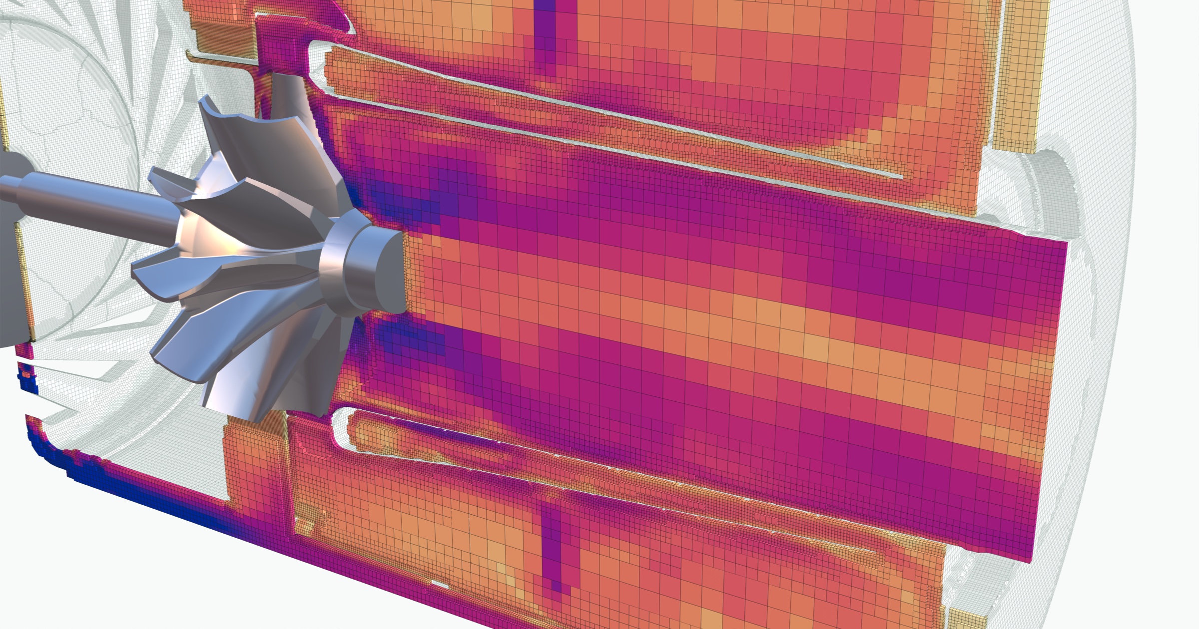
The air passages of a small turbojet, cut open along its axis, with each cell colored by flow speed.
Nobody analyzes a simulation mesh in Snowflake, Databricks, or an Iceberg table despite it being a reasonable thing to expect to work. Those systems absorb massive datastreams like ledgers, sensor logs, and financial data, and a 3D mesh looks like one more datastream with coordinates in it. In this post we want to illustrate why data warehouse tools don’t fit physical world data and outline a bit of what we are building to solve this problem. Where we can, we reference the warehouses’ own documentation stating as much.
The image above is one of these meshes: 18.3 million cells filling the air passages of a small turbojet.
Earthmover wrote the version of this post for weather and climate data in Tensors vs. Tables, which inspired this one. Their data is laid out along array axes, so the neighbors of a value are the ones next to it in the array, even when the grid itself is curved. That data belongs in chunked arrays, and flattening it into rows costs up to 10x at query time. Arrays beat tables for grids like that. The physical world data we work with is another step past it: any cell can connect to any other.
This is the first post in a series on physical world data. This one covers what analysis on a mesh means and why tables and arrays can’t run it.
Maps and point clouds already fit
Spatial data has gone into general-purpose databases before. PostGIS put maps in Postgres, every major warehouse has a geography type, and a capability that once needed its own product became a column type. Part of it already has. The one 3D data type with a cloud-native format is the point cloud. COPC is “a LAZ 1.4 file that stores point data organized in a clustered octree,” readable by HTTP range request. It works because a point cloud has no connectivity. Each point is independent, so an octree over x, y, z is a complete index, and the lidar demos on Snowflake and Databricks all flatten to one row per point.
Meshes stayed out because of connectivity: the record of which points join up to form each cell. A point stands alone, so it can be a row. A mesh cell can’t be analyzed without its neighbors.
What a mesh is
Here is a real finite element mesh of a beam, loaded with PyVista. The mesh is tiny: 2,192 cells built from 3,537 points. Nearly all of the cells are hexahedra (boxes with eight corners), and four are wedges (triangular prisms with six).
In [1]: import numpy as np
   ...: import pyvista as pv
   ...: from pyvista import examples

In [2]: grid = examples.download_notch_stress()

In [3]: grid.points.shape
Out[3]: (3537, 3)

In [4]: grid.get_cell(0).point_ids
Out[4]: [3379, 2904, 3349, 2893, 179, 689, 331, 269]

In [5]: grid.get_cell(1).point_ids
Out[5]: [1846, 1336, 1694, 1756, 3379, 2904, 3349, 2893]

In [6]: np.unique(grid.celltypes, return_counts=True)
Out[6]: (array([12, 13], dtype=uint8), array([2188,    4]))

In [7]: grid.point_data['Nodal Stress'].shape
Out[7]: (3537, 6)
The code shows the four kinds of array a mesh is made of. Every physics solver stores them in some form:
- Points (
In [3]). One x, y, z per point. The coordinates are values, the same as a temperature. Nothing about them is an axis. - Connectivity (
In [4]andIn [5]). For each cell, the list of point ids at its corners. The lists are different lengths: a wedge takes six ids, a hexahedron eight, a curved 20-node hexahedron twenty. - Cell types (
In [6]). One byte per cell naming its shape, so a reader knows how to interpret its list of ids. Here 12 is a hexahedron and 13 is a wedge. - Fields (
In [7]). The simulation’s results, stored per point or per cell. A field can be a scalar like temperature, a vector like velocity, or a tensor like the stress here, which has six components at each point.
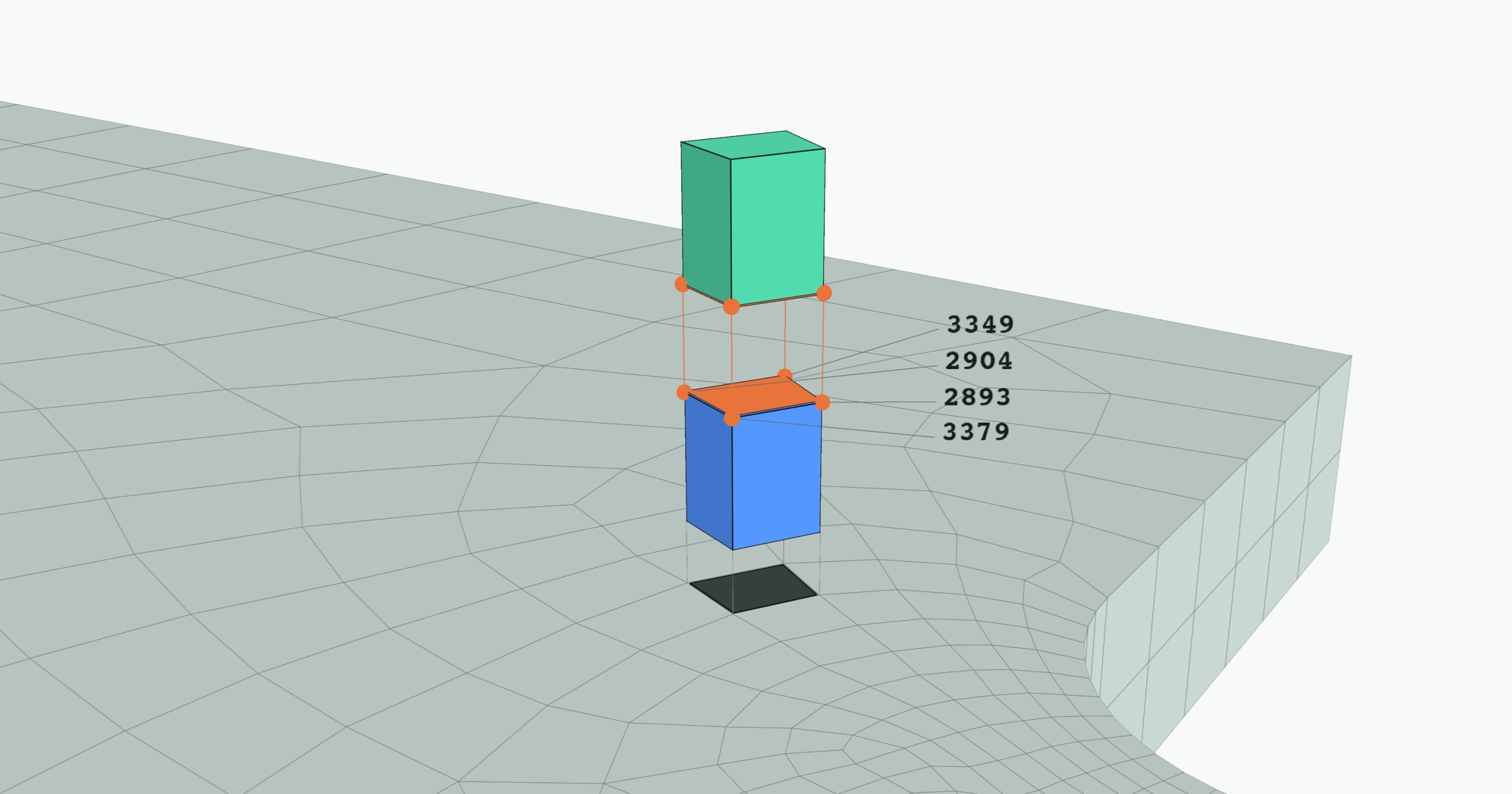
Compare Out[4] and Out[5]. Cells 0 and 1 both list points 3379, 2904, 3349, and 2893, so they share a face. Nothing stored in the mesh says these two cells are neighbors. The only way to find out is to compare their lists of point ids.
That makes a mesh a graph. On a grid, the neighbors of a cell follow from its index. In a mesh, cells are linked through the points they share, and those links have to be looked up. Every operation below starts with that lookup.
The cells don’t have to be straight either. Many solvers use cells whose edges are curves, defined by extra points along each edge and face. An array has no way to store that. It holds values at grid positions and says nothing about the shape of what lies between them. The probe section below shows what a curved cell changes.
What five common operations read from the mesh
Analysis on a mesh is a chain of transformations. In SQL, a filter keeps some rows and a join matches rows on a key. Both return rows built from values already in the tables. A mesh transformation reads the connectivity and writes a new mesh, often with points and cells that were not in the input.
The beam is too small to show much, so take a fluid simulation: two tubes of air merging into one, solved with OpenFOAM and shipped with PyVista’s examples. Its mesh has 400,712 cells of four types on 163,390 points.
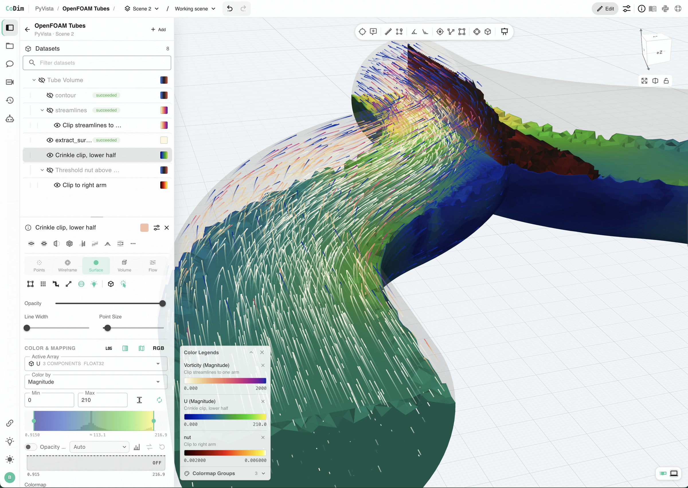
The sections below take five operations and cover what each one does and what it reads from the mesh, from the one closest to SQL to the one furthest from it.
Threshold: keep the cells that pass a test
Threshold keeps the cells where a field is above or below a value. It is the closest thing a mesh has to WHERE.
It is still a join. The field here is stored on points, and a cell passes if any of its points passes, so the test has to follow each cell’s list of point ids. The surviving cells use only some of the points, so the points are compacted and every id in the connectivity is renumbered. The output is a valid mesh again, with new ids.
Extract surface: find the outside
A solid mesh is mostly interior. To draw it or to read values on its surface, you need the faces on the outside. Extract surface finds them with one rule: an interior face is used by two cells, and an outside face is used by one.
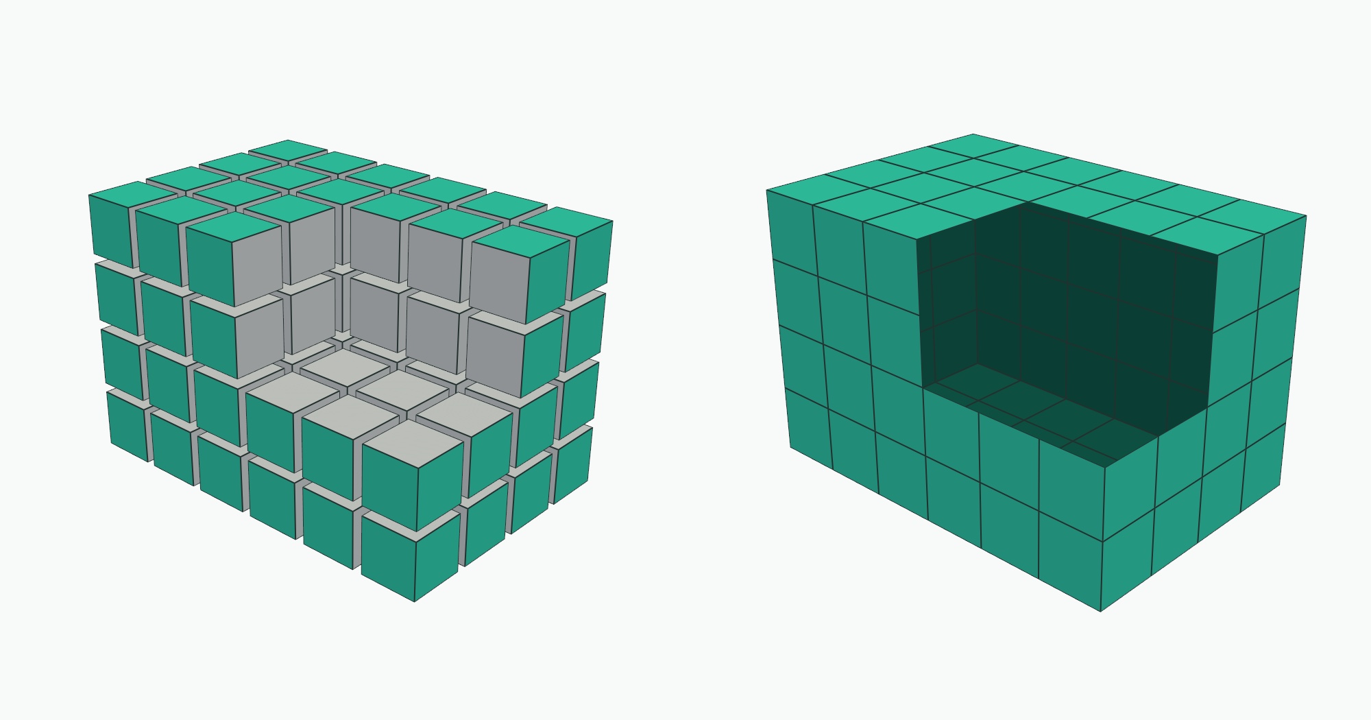
That is the shared-face question from the beam, applied to every face in the mesh.
Connected regions: split a result into its pieces
After a threshold, the surviving cells often form separate clumps: three hot spots or two cracks. A connected regions pass labels each clump so you can count them or measure them one at a time.
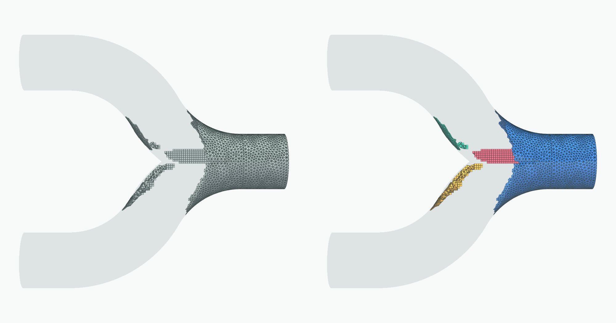
Two cells are in the same clump if they share a point, so the operation has to go from a point to every cell that uses it. The mesh only stores the direction from a cell to its points. A point-to-cell index has to be built first, and it is roughly as large as the connectivity array itself.
Clip and contour: cut through cells
Clip cuts the mesh with a plane and keeps the solid on one side. A contour is the cut on its own, at any value of a field: the surface where pressure is exactly 2 bar, or temperature exactly 600 K.
Both pass through the middle of cells, so their points are new. Wherever an edge has one end below the value and one end above, the operation puts a point partway along it, placed by interpolating between the two ends. Then it joins those points into triangles or smaller cells, using a lookup table of cut patterns for that cell type.
Neighbors also have to agree: two cells that share a cut face must split it the same way, or the output has cracks.
Probe: the value at a point
The most basic question anyone asks of a simulation is the value of a field at a spot in space. In a table with a spatial index that is a lookup. In a mesh, a probe is three steps.
Step one is the only step a spatial index helps with. Bin the bounding box of every cell, and ask which boxes contain the point. That is as far as a warehouse’s R-tree, S2 cell, or H3 index can take you.
Step two is finding where the point sits inside the cell. For a straight-edged tetrahedron that is one small linear solve. For anything with curved or twisted faces there is no formula. The lookup guesses a position, checks how far off it is, corrects, and repeats. That usually takes a few rounds, and it is capped at 10 or 20 per candidate cell.
Step three is blending the values at the cell’s corners. The value at the point is a weighted sum of the values stored on the cell’s points. The weights come from step two, and the formula for them depends on the cell type.
The bounding box in step one is only a hint, and curved cells show why. Build one on the unit cube and push the middle of one face outward by half a unit. Every corner still has x ≤ 1. Then ask whether the point (1.25, 0.5, 0.5) is inside it.
In [8]: cell = examples.cells.LagrangeHexahedron(cell_order=3)  # 64 points on the unit cube
   ...: on_face = np.isclose(cell.points[:, 0], 1.0)
   ...: interior = ((cell.points[:, 1] > 0.1) & (cell.points[:, 1] < 0.9)
   ...:             & (cell.points[:, 2] > 0.1) & (cell.points[:, 2] < 0.9))
   ...: cell.points[on_face & interior, 0] += 0.5   # bow the +x face outward

In [9]: corners = examples.cells.Hexahedron()       # the same eight corners, straight edges
   ...: query = [1.25, 0.5, 0.5]

In [10]: cell.find_containing_cell(query), round(cell.volume, 4)
Out[10]: (0, 1.2222)

In [11]: corners.find_containing_cell(query), round(corners.volume, 4)
Out[11]: (-1, 1.0)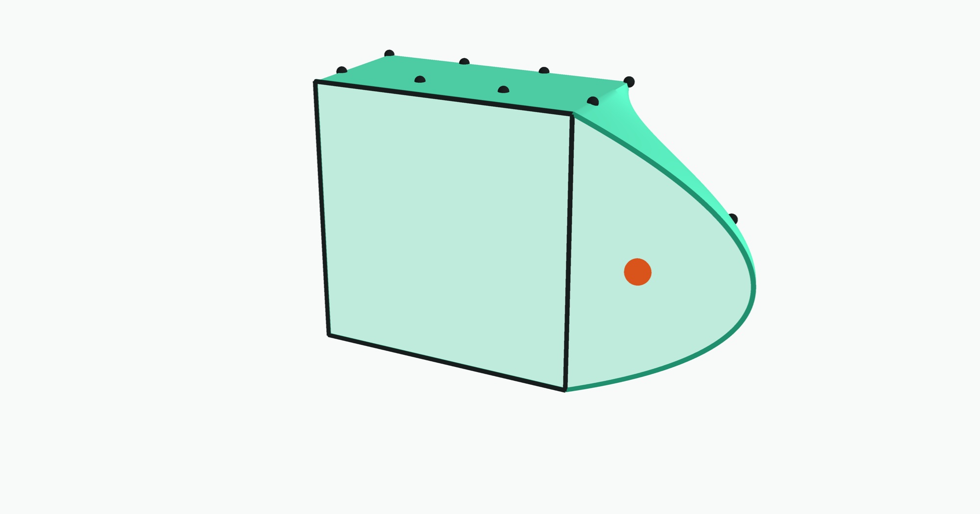
The curved cell contains a point that sits outside the box around its corners, and it has over 20% more volume than the straight-edged cell on the same corners. A system that models the cell as its eight corners gets both the containment and the volume wrong.
Curved cells are common. The structural solver Abaqus ships 20-node bricks and 10-node tetrahedra as standard element types. The flow solver Nek5000 represents its solution with polynomials of order 8 to 16 inside each element and states that “the geometry x is represented by high-order polynomials” too.
What the five have in common
Put the five side by side and mark what each one reads.
The list goes on past five. A gradient needs the geometry of every cell and the point-to-cell index. A streamline is a few hundred probes in a row, each one starting where the last ended. Integrating a field over a volume needs every cell’s volume, which is a different formula for each cell type. All of them read the same things: the connectivity, the cell type, and the geometry inside each cell.
What tables and arrays can and can’t hold
Tables and arrays each hold one kind of mesh completely.
- A table holds a mesh with no connectivity. That is a point cloud. Every point is independent, so one row per point loses nothing.
- An array holds a mesh whose connectivity follows from the index. That is a regular grid. The neighbors of a value are the ones next to it on each axis. Weather, climate, and imaging data have that shape.
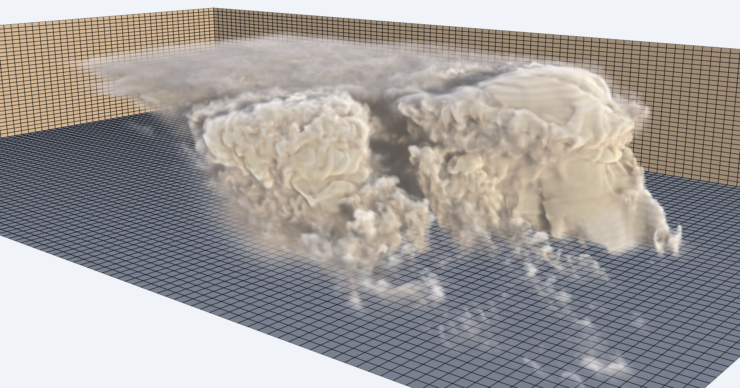
A general simulation mesh is neither. Its cells have mixed types, any cell can connect to any other, and some are curved.
A table can store it but not run on it. Flatten the mesh to one row per point and one row per (cell, corner) pair, and SQL can join those rows. That covers the first three columns of the matrix above, with every neighbor question a self-join on point id. The other columns have no SQL form: cut patterns per cell type, interpolation inside a cell, and cell geometry. Warehouse geometry types don’t fill the gap. They are map shapes, and the documentation for Snowflake, BigQuery, Redshift, Databricks, DuckDB, and PostGIS each says a third coordinate is rejected or ignored by most spatial functions. Microsoft Research’s finite element work on SQL Server in 2005 stored every tetrahedron as four rows and did the geometry outside the database. A 2014 paper that tried both relational and graph databases concluded that “since neither graph databases nor relational databases provides advanced geometric algorithms, we need a mesh library with geometric algorithms.”
An array has no axis to put it on. The only axis a general mesh has is cell number, which is whatever order the mesher or solver wrote the cells in. Position along it says nothing about which cells touch. The people who designed array databases drew this line themselves. The 2009 SciDB design paper scoped meshes out by name: “users with solid modelling applications want a mesh data model and will be unhappy with tables or arrays.” The authors chose arrays “because it makes a considerable subset of the community happy and is easier to build than a mesh model.”
A later post will go deeper on how specific warehouses and array formats handle this data.
What we are building instead
The operations above are solved problems on one machine. They have been open source for decades, and PyVista makes each one a single call. Desktop and cluster tools run them for one person in one session. What is missing is a service that runs them against meshes in object storage.
That is what CoDimensional builds. CoDim keeps each mesh in object storage with its connectivity intact. An analysis service runs next to that storage, built to spread the work across machines as meshes grow. You describe a pipeline, such as a clip followed by a threshold and streamlines. The service runs it on the full mesh, and what comes back is the result: a surface to draw, a number, a set of lines.
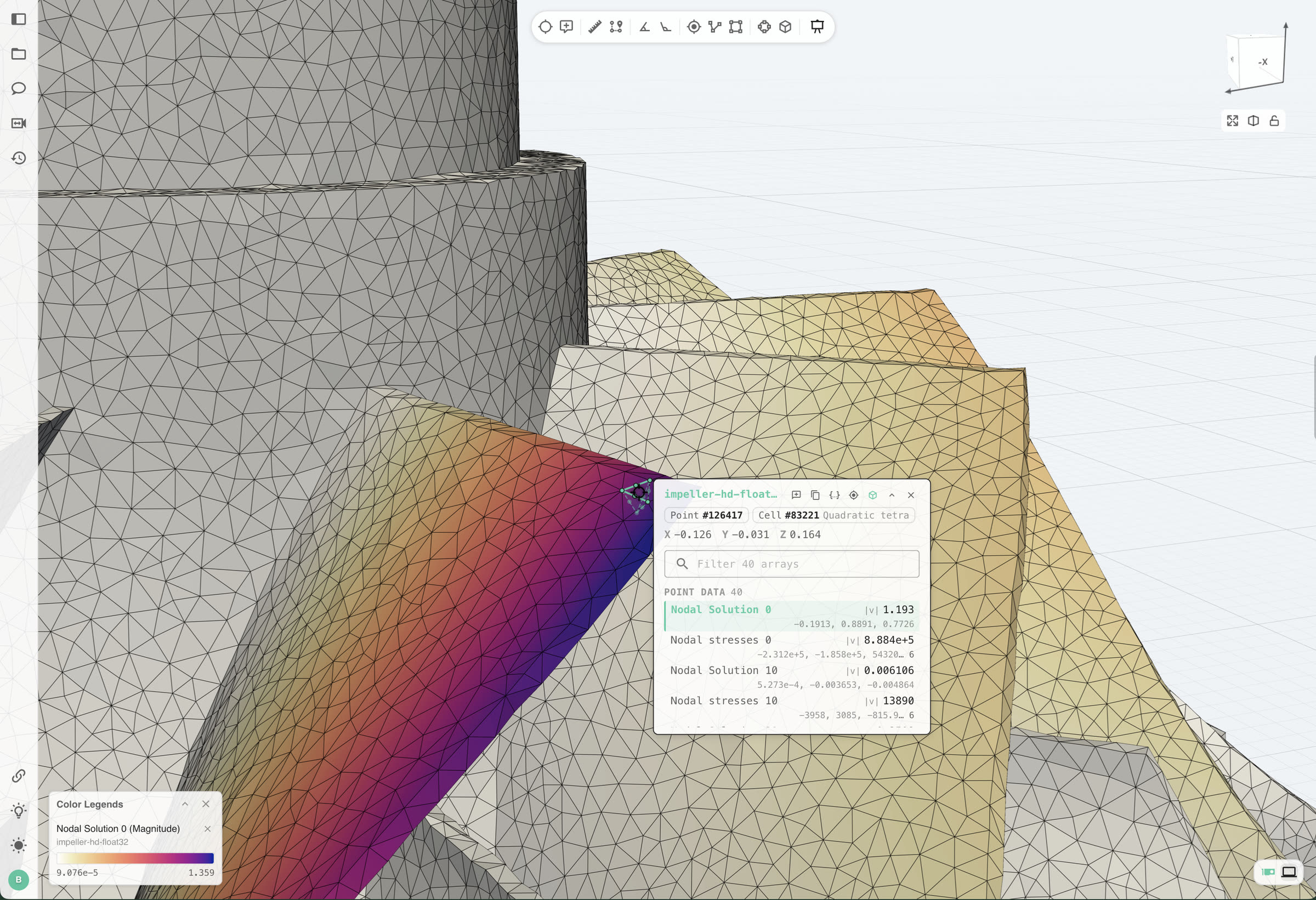
The analysis always runs on the mesh the solver wrote. A browser draws flat triangles, so what it receives is a simplified surface. A probe on that surface still answers for the source: click a triangle, and the readout names the original cell behind it, its type, and every field value at that point.
If you have a mesh that broke a table, bring us your data. We will run your analysis on it in CoDim and connect an agent to it, so you can ask it questions directly.
Get new posts by email